Real Projective Space

The real projective space ${\mathbb{RP}}^n$ is the set of all one dimensional subspaces of ${\mathbb{R}}^{n+1}$. This note deals with the construction of such a set, its parameterisation and intuition.

${\mathbb{RP}}^1$

${\mathbb{RP}}^1$ is the set of all one dimensional subspaces of ${\mathbb{R}}^2$. That is, the set of all lines through the origin in the two dimensional real coordinate space.

Homogeneous Coordinates

There are many ways we can parameterise such a set, one of which is using what are called homogeneous coordinates, which are vectors whose span is the desired one dimensional subspace, unique up to a scalar multiple.

Specifically, we define the equivalence relation $\sim$ where $(a,b)\sim (a^{\prime },b^{\prime })$ if and only if $(a,b)=\lambda (a^{\prime },b^{\prime })$ with $\lambda \in \mathbb{R}-\{0\}$, for $(a,b)\ne (0,0)$.

The homogeneous coordinates for the equivalence class containing $(a,b)$ are denoted by $[a,b]$, and therefore, for example $[1,2]$ refers to the same one dimensional subspace of ${\mathbb{R}}^2$ as $[2,4]$.

Gradient

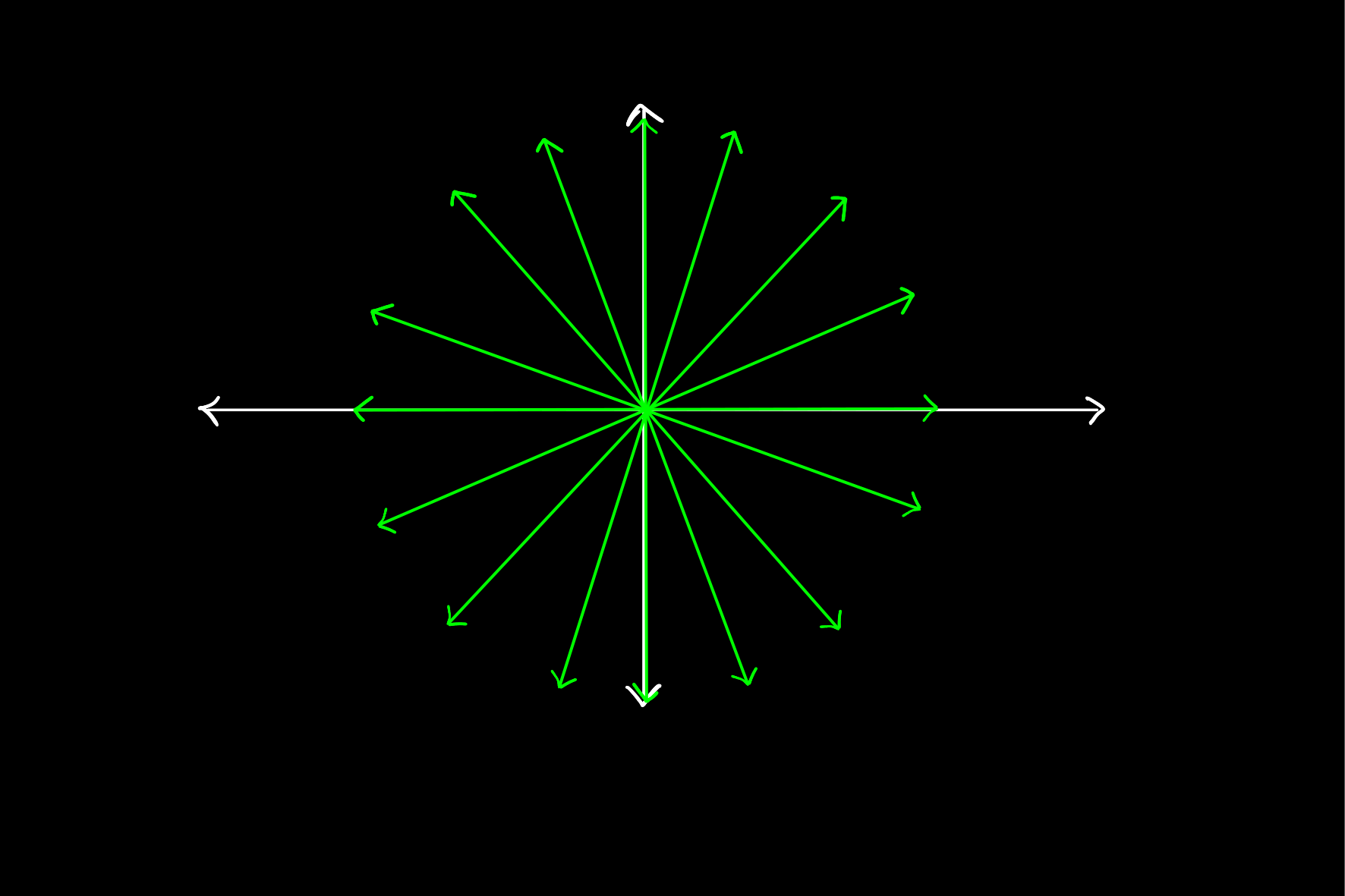
Another way is to use the gradient of the line, which assigns a unique real number to each one dimensional subspace of ${\mathbb{R}}^2$, with the exception of the $x=0$ line which we define with an infinite gradient. That is, there is a one to one correspondence between:

given by:

As the Unit Half Circle

The one dimensional subspaces of ${\mathbb{R}}^2$ are individual elements of ${\mathbb{RP}}^1$, and called projective points. ${\mathbb{RP}}^1$ is a one dimensional collection of projective points and is therefore called the real projective line.

This is because of the one to one correspondence that projective points have with half of the unit circle.

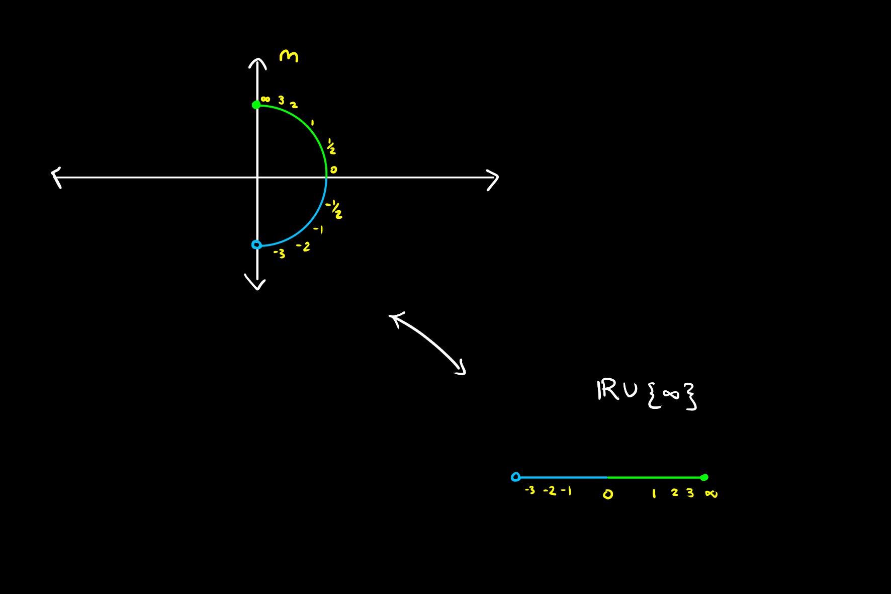
This is where the name projective space comes from. Every point in ${\mathbb{R}}^2$ is projected onto the unit half circle, and thus an entire one dimensional subspace appears as a single point. This intuition is stronger in the case of ${\mathbb{RP}}^2$ below.

${\mathbb{RP}}^2$

Again directly from the definition, ${\mathbb{RP}}^2$ is the set of all one dimensional subspaces of ${\mathbb{R}}^3$. That is, the set of all lines through the origin in the three dimensional real coordinate space.

Homogeneous Coordinates

We can similarly parameterise projective points in ${\mathbb{RP}}^2$ using homogeneous coordinates, in this case with three real numbers. That is, $[a,b,c]$ is the projective point in ${\mathbb{RP}}^2$ which corresponds with the one dimensional subspace of ${\mathbb{R}}^3$:

As ${\mathbb{R}}^2$ with the Projective Line

There is a one to one correspondance between:

given by

As the Unit Half Hemisphere

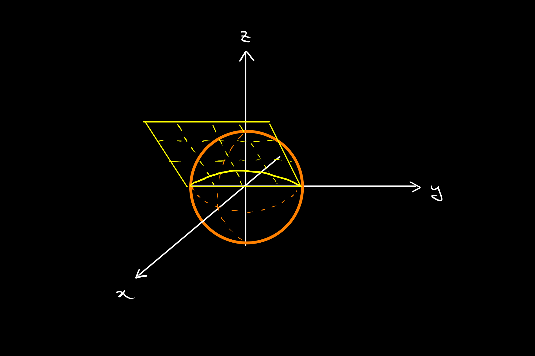
The parameterisation by homogeneous coordinates allows viewing the set of projective points in ${\mathbb{RP}}^2$ as points on the unit hemisphere in ${\mathbb{R}}^3$, analogous to the unit half circle in ${\mathbb{R}}^2$ for ${\mathbb{RP}}^1$.

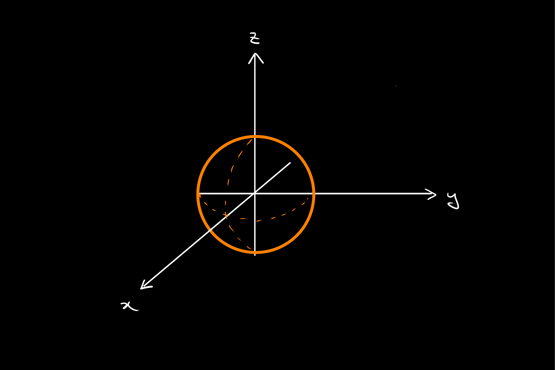
Thinking projectively, imagine being at the origin, and looking along the $x$ axis into this hemisphere. All of the points on a given one dimensional subspace of ${\mathbb{R}}^3$ appears as a single projective point from this perspective, collapsing everything in that space in on itself.

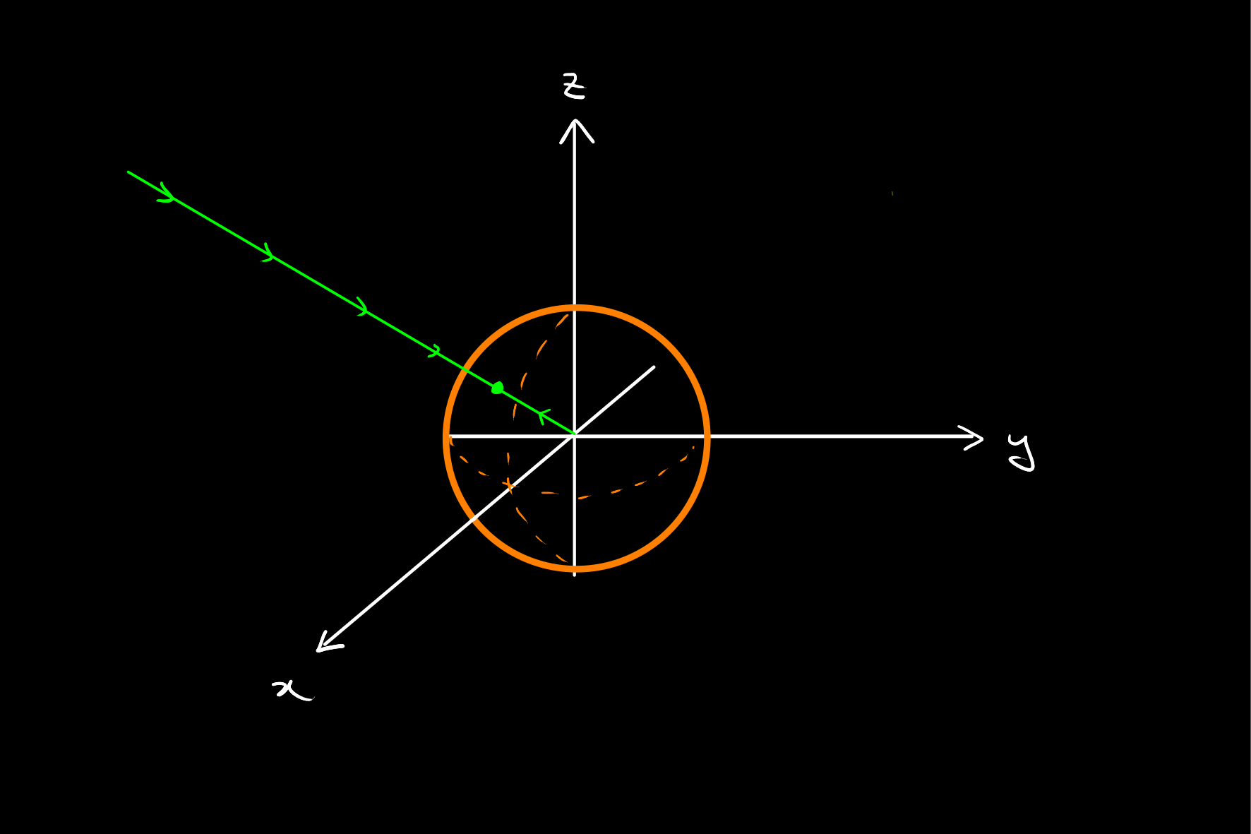
Similarly, a plane in ${\mathbb{R}}^3$, when collapsed in on the unit half hemisphere appears as a line from this perspective.

For example, ${\mathbb{RP}}^1$ is a projective line embedded in ${\mathbb{RP}}^2$.

Projective lines are often parameterised as the orthogonal complement of the one dimensional subspace represented by a projective point. That is, $[a,b,c{]}^{\perp }$ is the projective line corresponding with the subspace:

analogous to the point normal form of a plane.

Coincident Line

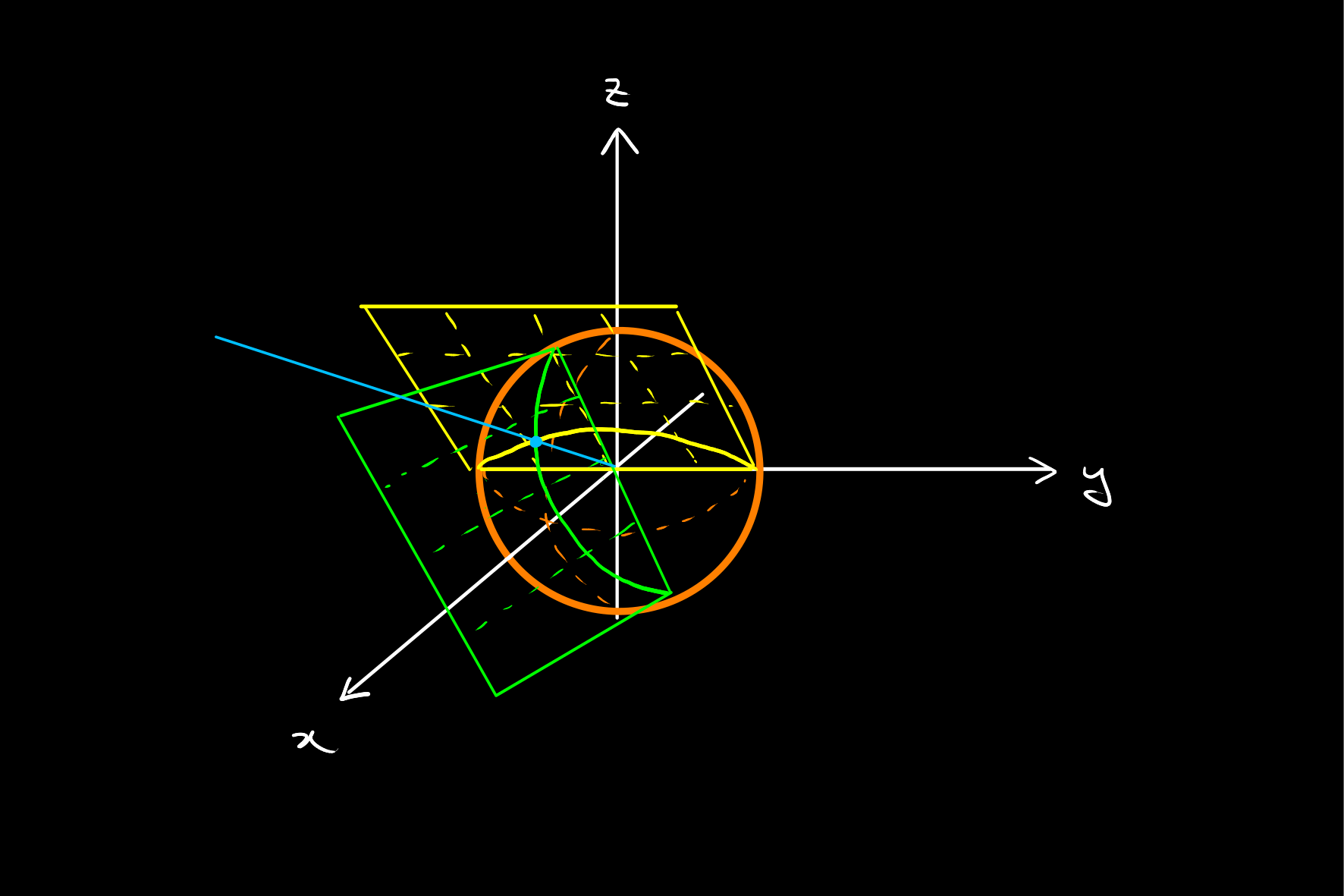
Given any two distinct projective points, which represent one dimensional subspaces of ${\mathbb{R}}^3$, there is a unique projective line which contains them, which corresponds to the plane containing both subspaces.

Hence finding the projective line through two projective points is a matter of taking a cross product.

For example, the projective line through $[1,3,2]$ and $[1,1,2]$ is calculated as:

and therefore given by $[4,0,-2{]}^{\perp }$.

Intersection of Lines

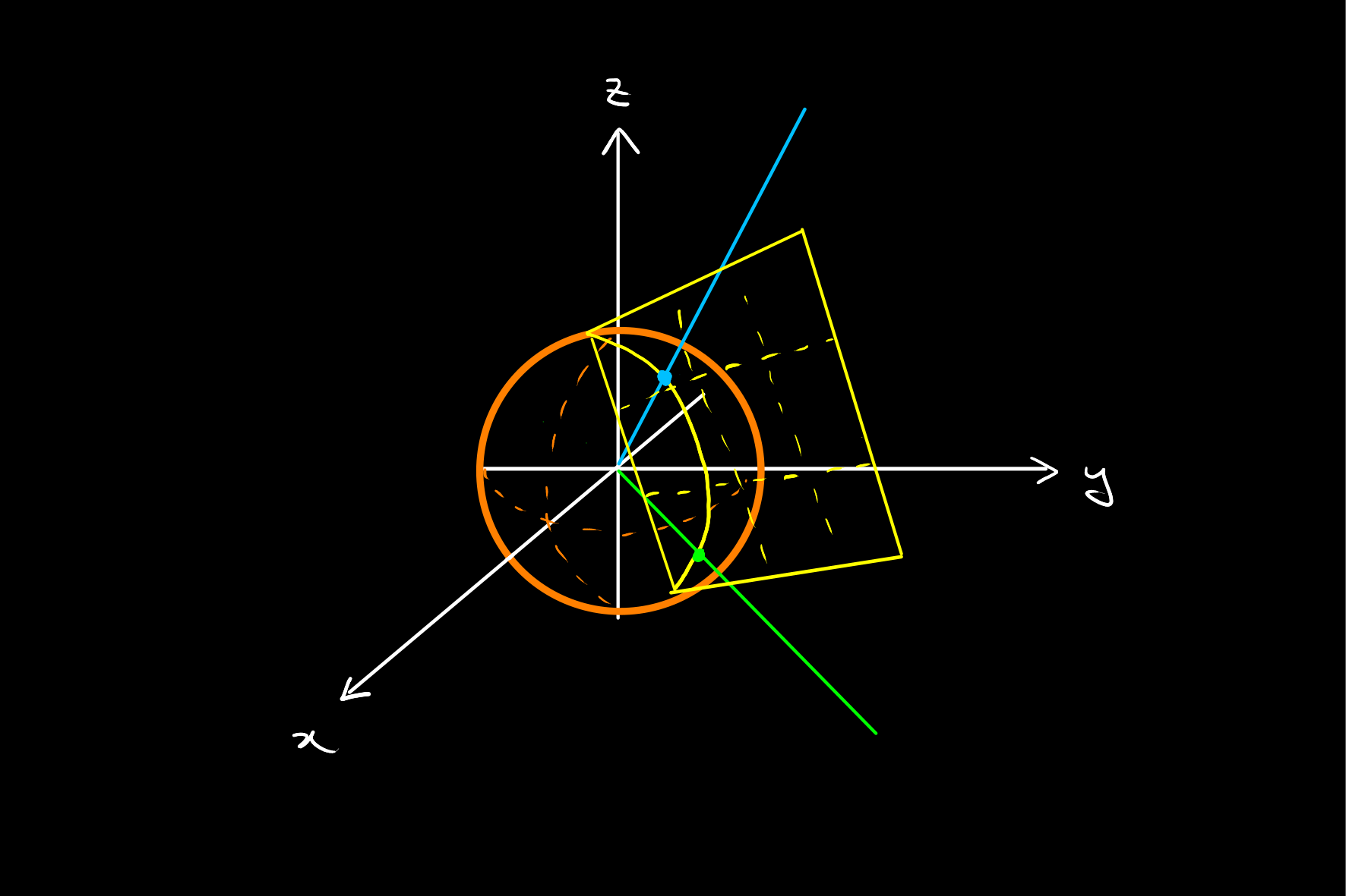
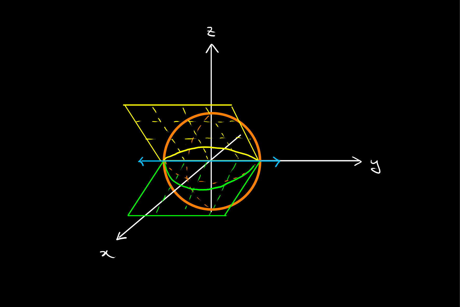
Given any two distinct projective lines, there is a single projective point at their intersection.

In this below example, the projective point in blue lies at the intersection of the yellow and green projective lines.

Similarly to the case of calculating the projective line through two projective points, calculating the intersection of two projective lines is just a cross product calculation.

Line at Infinity

The set of points of the form $[0,b,c]$ (the second case of the above map) are called the points at infinity because they lie on the line at infinity ${\ell }_{\mathrm{\infty }}=[1,0,0{]}^{\perp }$.

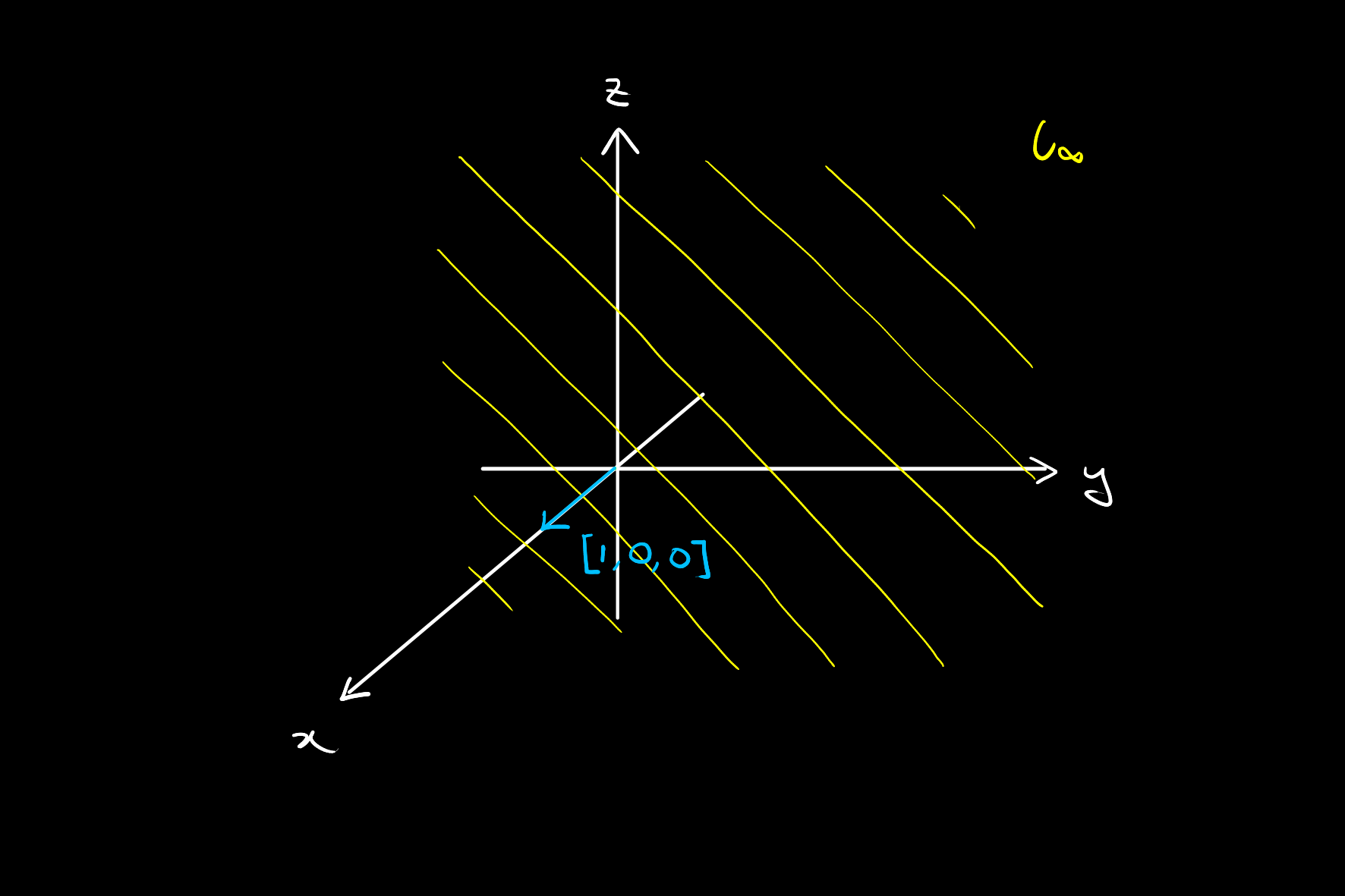
Every line which is not ${\ell }_{\mathrm{\infty }}$ has a single point at infinity.

Affine Points

The points which are not points at infinity are called affine points. This means their first component is non-zero, and hence can be written as $[1,y,z]$ for some $y,z$.

Corresponding Euclidean Line

A given projective line $[a,b,c{]}^{\perp }$ corresponds with the two dimensional subspace of ${\mathbb{R}}^3$ which is the set of points $(x,y,z)$ satisfying $ax+by+cz=0$. If $(x,y,z)$ corresponds with a homogeneous affine point, we can set $x=1$ and hence get the line $by+cz=-a$. Hence each projective line which is not ${\ell }_{\mathrm{\infty }}$ corresponds with a Euclidean line plus the one point at infinity.

Parallel Lines

Two projective lines in the real projective plane are said to be parallel if they appear parallel from the projective perspective (looking outwards from the origin). Two distinct lines are parallel if and only if they meet at a point at infinity.

We can determine if two lines are parallel by checking if the $x$ coordinate of their intersection is zero.

This means that the two lines $[a_1,a_2,a_3{]}^{\perp }$ and $[b_1,b_2,b_3{]}^{\perp }$ are parallel if and only if $a_2{b}_3-a_3{b}_2=0⟺\frac{a_2}{a_3}=\frac{b_2}{b_3}$.

This means their corresponding Euclidean lines are parallel in the normal geometric sense.

One can think about these parallel lines as like longitudinal lines, which meet only at the poles.

${\mathbb{RP}}^n$

The above ideas generalise to ${\mathbb{RP}}^n$, where points still represent one dimensional subspaces of ${\mathbb{R}}^{n+1}$, and each higher dimensional object in that space is constructed from sets of points.